Choosing the right chart task

Choosing the right chart

In this task you will be deciding which type of chart is most suitable to display all of parts of the various figures shown.

1. How people spent their time!

Make a chart to show how one of these people spend their time.


Make a chart to compare how much time all 5 people spend on eating.

Make a chart to compare how each person's day is spent.

2. Student results

Make a chart to compare how these 5 students did in each subject.

3. Progress with jobs

Make a chart to compare how these 5 people are progressing with the three jobs they have to do.

4. Profit and loss

[Click to enlarge this chart so you can read the data]

Make a chart to show the profit or loss for each month. Illustrate the difference between loss and profit months with a colour or effect.

Make a chart to show how the bank balance changes over the year.

Changes colours, fill effects, lines etc. to make these charts more attractive and clear. Make the final set of charts full size displays on their own sheets.

Name the sheets suitably and save the spreadsheet file.

How to make pictographs

Presenting information using pictographs 

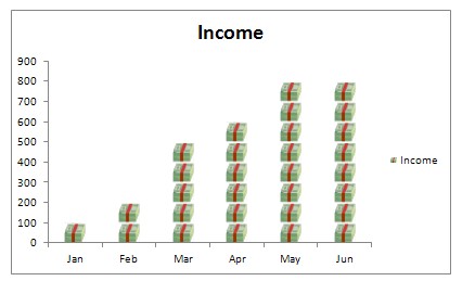
This is a way to display numeric information in an interesting way. It is a variation of a column or bar chart.

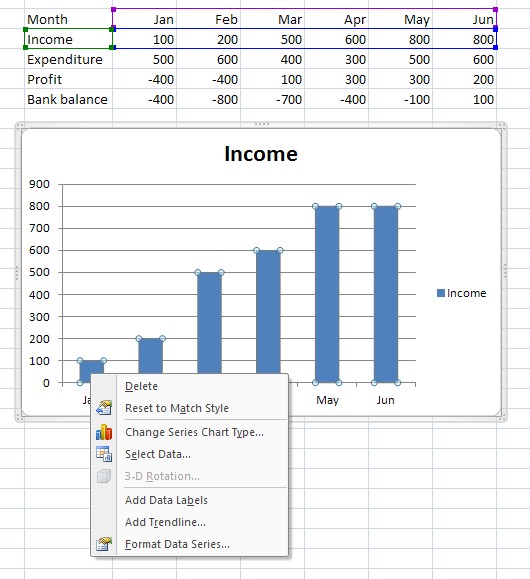
So instead of giving someone this type of information

You can show them this



Each bundle of notes represents 100.

How to make a pictograph in Excel (2007 or later)
1 Select the data required for a chart

2 Insert a bar or column chart (simple 2-D type)

3 Use whatever colours are provided and right click on any bar

 

4 Choose Format Data series.

5 In this panel choose Picture or texture fill, and Stack and Scale.

6 You will also need to choose an image to be used. Unless you already have something suitable, use the Clip Art option and search for an image. This can be changed later if you want to replace it with a better icon or picture from the web.

7 There are then three choices: Stretch, Stack, and Stack and Scale. The first, Stretch doesn’t usually work that well as it will make your image look strange! The best option is usually Stack and Scale where you also have to set a number for how many each image will represent. For example if you have small numbers in your data, like 2, 5 6, 11 then 1 unit per picture will work fine. If you have large numbers like 20000, 50000, 60000, 110000 then a unit of 10000 per picture would be better. In this example 100 units per picture has been used.

You may need to try a few different choices and see what works best with your data.

A different symbol has been used.

A change of scale is illustrated above. Note that in this option Excel will cut the image as appropriate where there an exact number will not match the data figures.

Peter's budget tasks

Peter is a carpenter. He makes kitchen cabinets and also does general building work. He is planning to introduce a new product – oak gazebos which are like permanent wooden tents people can have in their garden.

Your task is to help him work out how his cash flow will change over the year for different numbers of jobs that he hopes to get.

You are provided with a spreadsheet that has been partially completed. Download that at this link and save it.

1. You will need headings for the other months. Add February to December. (Remember, there is an easy way!)

2. Add a formula in cells G5 to G7 which will show the profit on each type of job. (Ignore other expenses at this stage, just take the cost away from the price)

3. Add the number of jobs he expects to get each month from this table.

4. Enter a formula to show the total number of jobs each month

5. Enter a formula to enter the income for January from each type of job. This will be the job price x number of jobs

6. Show the total income figures in row 20, the sum of the three figures above

7. In the Expenditure section, the cost of the Oak timber will be the number of Oak gazebo jobs x the Oak gazebo cost. Similarly, you can enter formulae to show Kitchen cabinet materials and General building costs.

8. Wages are for someone to help with the building jobs. He pays £100 per building job

9. The other expenses, drawings to sundry expenses, can all be assumed to be the same each month. Use either a formula or other method to copy these across.

10. Show the total expenditure figures in row 38.

11. The monthly profit will be his total income – total expenditure

12. The bank balance for January is entered already. From February it will be January’s balance + February’s profit. That formula can be copied for the other months.

13. Create a chart that shows Peter’s total jobs each month

14. Create a chart that shows his profit or loss for each month. Change the colours displayed so that the months with a loss stand out (eg profit in green, loss in red)

15. Create a chart that shows how his bank balance will change over the year.

16. Create three charts which indicate the cost and profit components of each type of job, expressing each as a percentage.

17. Copy the spreadsheet and display the formulae used.

Peter now wonders what would happen if he had to take July off too and would not be able to do any jobs that month. He realises that he will have to reduce his monthly drawings (what he pays himself each month) as it is important that he does not go overdrawn in December. By changing his monthly drawings determine the most he can pay himself each month and still be in the black at the end of the year.

Keep a separate copy of the chart showing this.

Output

• Sheet with complete data entered 
• A chart of total jobs each month 
• A profit and loss chart 
• A bank balance chart 
• Job cost / profit charts 
• Formulae sheet 
• Effect of July holiday and lower drawings chart

[Word version available here] | [Download the draft spreadsheet here]

Help with the Peter spreadsheet

Ideas!

1.       Entering months

drag the little black box at the corner across and the months will just appear
2.       Add a formula in cells G5 to G7 which will show the profit

=B5-E5 will work for Oak gazebo profit. That formula can be copied down with the same little black box for the other two.

3.       Add the number of jobs he expects to get each month from this table.
Just type in the right cells

4.       Enter a formula to show the total number of jobs each month
=SUM(B11:B13) will add the right figures for January. Again, copy across for other months

5.       Enter a formula to enter the income for January ..
You need to make sure the formula always uses the same Price for Oak gazebos. So use =$B$5*B11 (with those $ signs). That can then be copied across. It’s 0 for some months.
=$B$6*B12 will work for kitchens
=$B$7*B13 will work for building

6.       Show the total income figures in row 20, the sum of the three figures above
=SUM(B16:B19) will add the income for January and can be copied across

7.       In the Expenditure section, the cost of the Oak timber will be the number of Oak gazebo jobs x the Oak gazebo cost. Similarly, you can enter formulae to show Kitchen cabinet materials and General building costs.
=$E$5*B11 (with the dollar signs) is needed for January and can then be copied
=$E$6*B12 for kitchens
=$E$7*B13 for building

8.      Wages are for someone to help with the building jobs. He pays £100 per building job
=B13*100 will work and can be copied

9.       The other expenses, drawings to sundry expenses, can all be assumed to be the same each month. Use either a formula or other method to copy these across.
10.   Show the total expenditure figures in row 38.
Another Sum formula =SUM(B23:B37) will work and can be copied

11.   The monthly profit will be his total income – total expenditure
=B20-B38 will work and can be copied

12.   The bank balance for January is entered already. From February it will be January’s balance + February’s profit. That formula can be copied for the other months.
Put =B40 in the January balance column.
=B42+C40 will then work for February and can be copied across

13.   Create a chart that shows Peter’s total jobs each month
Highlight from A9 to M9 (the months row) then hold the Ctrl key and highlight A14 to M14
Then try Insert>Chart and choose a column type

14.   Create a chart that shows his profit or loss for each month. Change the colours displayed so that the months with a loss stand out (eg profit in green, loss in red)
again, start with A9 to M9, hold Ctrl and highlight A40 to M40
Then Insert >Chart and choose a column type
To change any bar colour, click any bar once and then click again so just one is selected
You can use the Fill or Shading button on the home toolbar to pick a colour. Repeat for others to be changed.

15.   Create a chart that shows how his bank balance will change over the year.
Select A9 to M9, hold Ctrl and then select A42 to M42
Insert>Chart and select a line type

16.   Create three charts which indicate the cost and profit components of each type of job, expressing each as a percentage.
Select A5, E5 and G5 using the Ctr method to skip other cells.
Insert>Chart and choose a pie chart

17.   Copy the spreadsheet and display the formulae used.
To copy the sheet, point to its tab with the mouse and then hold the Ctrl key down while you drag the tab to the right, release the mouse, then the Ctrl key. That should make a second copy with (1) after the tab name.
To show formulae use Ctr+` (the key to left of 1 on most keyboards). Don’t worry if the sheet looks odd!